Financial Architects

  • Home
  • About Us
  • Services
  • Resources
  • Ruminations Blog
  • Contact Us

November 1, 2017 by David E. Hultstrom

Evidence-Based Investing

We practice what is now being called “evidence-based investing” (description here for example) – so-called because sound academic research supports it.  This month I thought I would review the key findings of some of the seminal papers in the field. I present these in chronological order with a one-sentence summary in bold at the end of each synopsis:

Can Stock Market Forecasters Forecast? (1932) by Alfred Cowles III. He concluded:

Sixteen financial services, in making some 7500 recommendations of individual common stocks for investment during the period from January 1, 1928, to July 1, 1932, compiled an average record that was worse than that of the average common stock by 1.43 per cent annually. Statistical tests of the best individual records failed to demonstrate that they exhibited skill, and indicated that they more probably were results of chance.

Twenty fire insurance companies in making a similar selection of securities during the years 1928 to 1931, inclusive, achieved an average record 1.20 per cent annually worse than that of the general run of stocks. The best of these records, since it is not very much more impressive than the record of the most successful of the sixteen financial services, fails to exhibit definitely the existence of any skill in investment.

William Peter Hamilton, editor of the Wall Street Journal, publishing forecasts of the stock market based on the Dow Theory over a period of 26 years, from 1904 to 1929, inclusive, achieved a result better than what would ordinarily be regarded as a normal investment return, but poorer than the result of a continuous outright investment in representative common stocks for this period. On 90 occasions he announced changes in the outlook for the market. Forty-five of these predictions were successful and 45 unsuccessful.

Twenty-four financial publications engaged in forecasting the stock market during the 42 years from January 1, 1928, to June 1,1932, failed as a group by 4 per cent per annum to achieve a result as good as the average of all purely random performances. A review of the various statistical tests, applied to the records for this period, of these 24 forecasters, indicates that the most successful records are little, if any, better than what might be expected to result from pure chance. There is some evidence, on the other hand, to indicate that the least successful records are worse than what could reasonably be attributed to chance.

In other words, no, forecasters can’t forecast. (Mr. Cowles had a follow-up paper in 1944 as well which concluded much the same thing. See also The Fortune Sellers and The Signal and the Noise.)

Portfolio Selection (1952) by Nobel laureate Harry Markowitz. This landmark paper introduced what became known as Modern Portfolio Theory (MPT). With estimates of the expected returns and variances of investment opportunities, along with expected correlations between them, an optimal portfolio may be constructed that maximizes the expected returns for the risk taken or (identically) minimizes the risk for the expected return. Constructing an optimal portfolio is a mathematical, not creative, exercise.

Challenge to Judgement (1974) by Nobel laureate Paul Samuelson. He concluded, “What is interesting is the empirical fact that it is virtually impossible for academic researchers with access to the published records to identify any member of the subset with flair [the ability to outperform].” Active management doesn’t seem to win.

The Loser’s Game (1975) by Charles Ellis. He concluded, “[E]fforts to beat the market are no longer the most important part of the solution; they are the most important part of the problem.” The way to win (outperform) is not to lose (by incurring high costs).

Common Risk Factors in the Returns on Stocks and Bonds (1993) by Nobel laureate Eugene Fama and Ken French. This paper introduced what became known as the “three-factor model” for stocks (plus two, credit and term, for bonds). There is a return from owning stocks over bonds, plus a premium for smaller companies (earlier identified by Banz in 1980), plus a premium for less expensive (aka value) stocks (earlier identified by Basu in 1977). Despite these earlier papers from Banz and Basu, the 1993 Fama and French paper is much more widely cited. Value (cheaper) and smaller stocks tend to outperform.

The Arithmetic of Active Management (1991) by Nobel laureate William Sharpe. Passive investors own the market portfolio and thus earn the market return. Active investors, in aggregate, must own the market portfolio as well and thus will also earn (gross) the market return, but due to much higher costs will inevitably underperform (as a group) net. Active management can’t win.

Determinants of Portfolio Performance (1995) by Brinson, Hood, and Beebower. In a study of 91 large U.S. pension plans they determined that the strategic allocation to stocks, bonds, and cash was by far the crucial decision. Indeed, the decisions of which individual securities to buy or the decision to deviate tactically from the strategic allocation (presumably with the view that investments were cheap or expensive) removed value! In other words, if these pension plans had just selected an asset allocation, bought index funds to implement it, and rebalanced back to the target periodically, they would have had better performance. Pick an allocation, implement it cheaply, rebalance periodically and otherwise resist the temptation to “do something.”

On Persistence in Mutual Fund Performance (1997) by Mark Carhart. This paper added momentum (previously identified by Jegadeesh and Titmanto in 1993) to the small-cap and value factors previously identified by Fama and French (above) as leading to improved returns. Despite the earlier paper from Jegadeesh and Titmanto, the 1997 Carhart paper is much more widely cited. Investments that have done well (poorly) in the past year tend to continue to do well (poorly).

Despite all of these papers being at least two decades old, most of the industry persists in being “faith-based” instead of “evidence-based” – probably because the management fees are higher for hope! So let me summarize the whole thing:

  1. The most important thing is to get the allocation to stocks, bonds, and cash right and diversify appropriately.
  2. Trying to beat the market through timing or security selection generally doesn’t work and costs matter a great deal.
  3. Notwithstanding the previous point, systematically tilting a portfolio toward smaller companies (small-cap), cheaper companies (value), and investments that have done well recently (momentum) does appear to work (on average over time, of course).

Filed Under: uncategorized

October 1, 2017 by David E. Hultstrom

After-Tax Portfolio Allocations

In previous posts I have explored After-Tax Returns to Different Types of Accounts and Tax-Efficient Spending from a Portfolio.  In this post, I will expand a little further on how the type of account which holds an investment can affect the distribution of returns.

Advisors don’t generally consider the after-tax allocations of their clients’ portfolios for two reasons: first, because the complexity is very high and second, because clients don’t think in those terms.  Nevertheless, in theory, we really should use after-tax allocations.  Here is the simple version:

Assume an account value of $100, a tax rate of 25%, a return of 10%, and a standard deviation of 20%.  (The actual numbers selected aren’t important to my point.)

If the account is a Roth and the basis is anything lower than $100, the liquidation value is $100, the return is 10%, and the standard deviation is 20%.  (You are undoubtedly thinking, “duh” but stay with me.)

If the account is an IRA, and the basis is zero then the liquidation value is $75, and the return is 10%, and the standard deviation is 20%, both calculated on that $75 value, not on the $100 ostensible balance.

In other words $100 in stocks in an IRA and $100 in bonds in a Roth is really $75 in stocks and $100 in bonds.  (As you can also see if you considered a Roth conversion between the two buckets where the taxes are paid out of the IRA instead of an outside source.)  So it would be more logical for us to do asset allocations based on net after-tax values but as noted above clients don’t think in those terms.

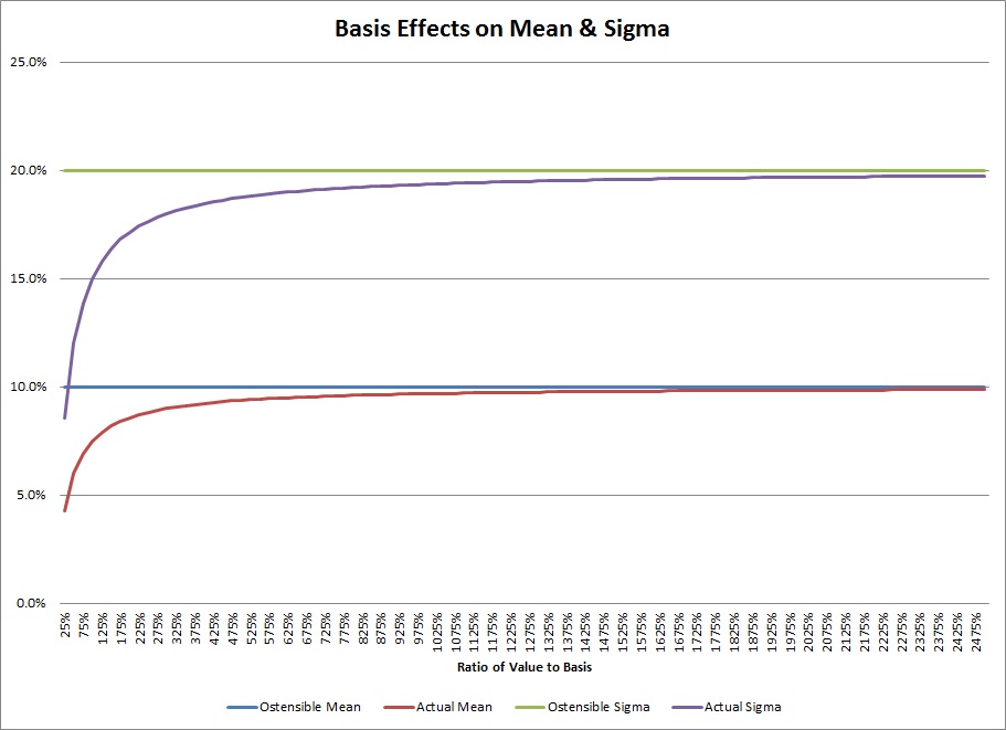
Now that is ugly enough, but it gets much, much worse if there is basis.  If there is no basis, the result would be at the far right of this graph (i.e. with no basis the ratio would be infinity and the ostensible and actual numbers would match.  Also note that the math is identical for a taxable account as well (though the rate would be cap gains rates).

So for an account or position where there are enormous losses (the left side of the graph above), oddly the true returns and standard deviations are much diminished (the higher moments of the distribution – skewness and kurtosis – are unchanged), but as the position or account increases in value the numbers asymptotically approach the stated values. Remember, these returns are from the liquidation value, not the number on the statement that has embedded taxes.  To tweak the example above, for all investments assume a 10% return, a 20% standard deviation, a 25% ordinary income bracket, and a 15% capital gains rate:

  • Assume a Roth with a basis of $100 and a value of $1,000.  It should be considered as an investment of $1,000 with a return of 10% and a standard deviation of 20%.
  • Assume an IRA with a basis of $500 and a value of $1,000.  It should be considered as in investment of $875 with a return of 8.57% and a standard deviation of 17.14%.
  • Assume a taxable account with a basis of $2,000 and a value of $1,000.  It should be considered as an investment of $1,150 with a return of 7.39% and a standard deviation of 14.78%.

These three “identical” investments in the three different accounts for one client would commonly be considered an investment of $3,000 with a return of 10% and a standard deviation of 20% but it is really an investment of $3,025 with a return of 8.59% and standard deviation of 17.19% (the weighted averages of the after-tax values).

Assume an astute financial advisor then harvests the loss in the client’s taxable account.  She saves $150 on her taxes (assuming there are other long-term gains to take it against) and then has a taxable account with a value of $1,000 and a return of 8.5% and a standard deviation of 17%.  Now the entire portfolio has a value of $2,875 with a return of 9.04% and a standard deviation of 18.09%.  Harvesting losses increases risk and return while lowering the initial value of the portfolio (because the tax savings has been realized).

Filed Under: uncategorized

September 1, 2017 by David E. Hultstrom

After-Tax Returns to Different Types of Accounts

Let’s assume five different types of accounts are available:

  1. A taxable account where the funds are withdrawn to spend during life
  2. A taxable account where the funds are left for heirs
  3. A deductible IRA (or 401(k), 403(b), etc. the math is the same)
  4. A Roth (or again a Roth 401(k), 403(b), etc. the math is again the same)
  5. A non-deductible IRA

Let’s further assume:

  1. The tax treatment of a Roth remains the same (i.e. tax fee growth).
  2. Investments held until death continue to receive a step up in basis as they do currently.
  3. The investment throws off no dividends or interest and there is no portfolio turnover during the holding period.
  4. There are no RMDs (Required Minimum Distributions) on any accounts.

Interesting and notable (and counter-intuitive to most folks) findings:

  • The rate of return is actually completely irrelevant to which investment is superior, but it will increase the magnitude of the differences between the different types.
  • If the ordinary income tax rate remains the same – regardless of the level – it is a three way tie between the deductible IRA, the Roth, and the taxable account held until death.
  • If the ordinary income tax rate increases, it is a two way tie between the Roth and the taxable account held until death.
  • If ordinary income tax rates decrease, the deductible IRA wins.
  • The non-deductible IRA never wins under any circumstance (with my assumptions, but with dividends, interest, and turnover it can beat a taxable account).
  • The taxable account never wins, but if capital gains rates are low enough, it can beat the deductible IRA in the case where ordinary income rates increase significantly (for example, if capital gains rates are 20% and ordinary rates are currently 25%, but go to 37.5% it will be a tie.  If they increase to above 37.5%, the taxable account would win).  But note that the Roth would have beat both by a wide margin.

Filed Under: uncategorized

August 1, 2017 by David E. Hultstrom

Changing Income Tax Rates

There are two contradictory forces and one inefficiency at work when income tax rates are changed:

  • First, there is the familiar Laffer Curve effect which effectively says as you increase taxes on labor people substitute untaxed leisure.  I.e. you get less of what you tax.  That is fairly uncontroversial as a theoretical construct, but there is little agreement on how large the effect is.  It can be called the substitution effect.
  • Second, there is a countervailing effect called the income effect.  If people need a certain amount of money to live then arguably raising tax rates (thus reducing their consumable income) could lead them to work more to get the same amount of money.
  • Third, the inefficiency is that at high rates people may do economically inefficient things to avoid the taxes (hold on to things to avoid capital gains taxes, use non-qualified deferred comp, put more in retirement plans than they would otherwise, set up a C corp. and retain the earnings in that entity, etc.) those are considered inefficient because it isn’t what people would choose to do absent the high taxes so there is a reduction in utility.

All of these effects will hit different people and items differently.  Here are a few of the main ones:

  • Low-income workers – the income effect will probably dominate so raising taxes on the relatively poor or lower middle class is a very good way to raise revenue (I am not necessarily recommending it, I’m just sayin’…).  They can’t afford to work less, and have few options for avoiding the tax aside from taking cash jobs off-the-books.
  • High-income workers – in theory the substitution effect should dominate, but it doesn’t appear to (with one exception I’ll get to next).  That may simply be that we haven’t had rates high enough to trigger it.  The rates necessary to make raising taxes unproductive (Laffer Curve maximum) might be as high as 60-70% though you still would create drag on the economy even below those rates.  In other words, if taxes are raised 10% and that causes a 5% reduction in hours worked for the group, tax revenue is increased but GDP will be lower so the economy isn’t doing as well overall.  High-income workers also have more flexibility to take income as perks or in different forms, delay recognition, move out of the country, etc. so the third item (inefficiency) from above is important here as well.
  • High-income worker married to a low-income worker – the data does show that the lower paid spouse does tend to opt out of the paid labor force with higher taxes.  For example, a lower income spouse might stay home at higher rates.  That is bad for tax receipts, but also bad for lower-income workers if in staying home tasks are no longer outsourced.  In other words, he or she might cook more rather than the family eating out, clean more rather than hire a maid, mow the lawn more rather than hire a lawn service, wash and iron clothes more reducing the need for dry-cleaning services, and watch the kids more reducing the need for daycare.  Thus, by raising taxes on “the rich” it could reduce government revenue while simultaneously reducing the income of waitresses, cooks, maids, gardeners, drycleaners, childcare workers, etc. – none of whom are likely to be “rich.” For example, suppose the marginal tax rate on our taxpayer was 50% but it is raised to some higher amount while these other lower-income workers are in the 25% bracket the entire time.  The lower-paid spouse did make $40,000 which after tax was $20,000 which was all spent paying for these additional services.  The government got $20,000  plus $5,000 from the other folks.  By staying home and doing all these things “in house,” spendable income (on other things) is exactly the same – there is no loss of standard of living (though of course the stay-at-home spouse may disagree) – but the government is out $25,000, and low paid workers out $15,000.
  • Recognition of capital gains taxes is frequently very discretionary and thus even modest increases in this rate probably triggers more of a Laffer Curve effect.  It is hard to see how there would be any income effect at all.

So what is the conclusion?  Assuming Congress is rational (so already this is silly conjecture) there should be a trend to:

  • Raising taxes on lower incomes.
  • Keep capital gains taxes low (and though I didn’t touch on it here, dividends as well because an unpaid dividend becomes a capital gain eventually, and we don’t need further incentives for debt in the capital structure of companies).
  • Change the code to treat each person individually rather than as a household (i.e. you may be married, but each spouse still files an individual return).  This has the advantage of not treating unmarried couples differently and allows the lower-income spouse to have a low marginal rate and thus stay in the workforce.
  • Raise taxes on higher incomes modestly.  There is probably room before the Laffer Curve maxes out – particularly if the previous bullet is implemented.

Filed Under: uncategorized

July 1, 2017 by David E. Hultstrom

How We’re Different

I read Different a few years ago and highly recommend it.  I thought about our business and how we are different from “wirehouse brokers” (i.e. large firms), and I made this list:

  • We have no idea what the Dow did today, nor do we think it is important.
  • We are bad at sales and good at expertise.
  • We don’t have any proprietary products, principal transactions, commissions, sales contests, etc.
  • We will give tax advice.
  • We don’t call clients for permission to make a change in their accounts just to avoid fiduciary liability.
  • We know what we don’t know – as far as I know. 🙂
  • We don’t segment clients into gold, silver, lead categories and give different levels of service accordingly.  Every client we accept is a platinum client.
  • We don’t “cross sell” mortgages, insurance, etc.
  • We won’t sell clients what they want if we don’t think it is prudent.
  • We aren’t pushing the “hot” product just because it has a great story (IPOs, growth stocks, commodities, gold, hedge funds, other alternative investments).
  • We won’t let clients draw too much from their portfolios even though it will make them happy now (because they will be unhappy decades from now).
  • We want to know the client’s entire financial situation and won’t take them as a client otherwise.
  • We  won’t buy and sell in client portfolios just to look like we are doing something.
  • We won’t provide clients our quarterly performance compared to a benchmark – it isn’t relevant.
  • We are expensive for small clients and cheap for large ones.
  • We frequently aren’t in the office, and when we are we aren’t watching CNBC or quote screens.
  • We make our own decisions.
  • We don’t have Class A office space (or expenses).
  • We ignore “hot” managers and great track records.
  • We don’t sell individual securities.
  • We pay attention to taxes and costs.
  • We won’t be going golfing with clients (but lunch is great!)
  • We have clients all over the country rather than just near our office.

Filed Under: uncategorized

  • « Previous Page
  • 1
  • …
  • 18
  • 19
  • 20
  • 21
  • 22
  • …
  • 32
  • Next Page »

Join Our List

Sign up to receive our newsletter "Financial Foundations" and stay informed of important financial planning and wealth management strategies.

  • This field is for validation purposes and should be left unchanged.

Recent Posts

  • Tax Opportunities
  • Three More Mental Mistakes
  • Summer Ruminations
  • Two Mental Mistakes
  • Why We Don’t Invest in Alts
  • Disclaimer
  • Disclosure
  • Form ADV
  • Privacy