In previous posts I have explored After-Tax Returns to Different Types of Accounts and Tax-Efficient Spending from a Portfolio. In this post, I will expand a little further on how the type of account which holds an investment can affect the distribution of returns.
Advisors don’t generally consider the after-tax allocations of their clients’ portfolios for two reasons: first, because the complexity is very high and second, because clients don’t think in those terms. Nevertheless, in theory, we really should use after-tax allocations. Here is the simple version:
Assume an account value of $100, a tax rate of 25%, a return of 10%, and a standard deviation of 20%. (The actual numbers selected aren’t important to my point.)
If the account is a Roth and the basis is anything lower than $100, the liquidation value is $100, the return is 10%, and the standard deviation is 20%. (You are undoubtedly thinking, “duh” but stay with me.)
If the account is an IRA, and the basis is zero then the liquidation value is $75, and the return is 10%, and the standard deviation is 20%, both calculated on that $75 value, not on the $100 ostensible balance.
In other words $100 in stocks in an IRA and $100 in bonds in a Roth is really $75 in stocks and $100 in bonds. (As you can also see if you considered a Roth conversion between the two buckets where the taxes are paid out of the IRA instead of an outside source.) So it would be more logical for us to do asset allocations based on net after-tax values but as noted above clients don’t think in those terms.
Now that is ugly enough, but it gets much, much worse if there is basis. If there is no basis, the result would be at the far right of this graph (i.e. with no basis the ratio would be infinity and the ostensible and actual numbers would match. Also note that the math is identical for a taxable account as well (though the rate would be cap gains rates).
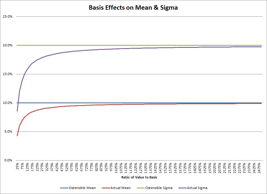
So for an account or position where there are enormous losses (the left side of the graph above), oddly the true returns and standard deviations are much diminished (the higher moments of the distribution – skewness and kurtosis – are unchanged), but as the position or account increases in value the numbers asymptotically approach the stated values. Remember, these returns are from the liquidation value, not the number on the statement that has embedded taxes. To tweak the example above, for all investments assume a 10% return, a 20% standard deviation, a 25% ordinary income bracket, and a 15% capital gains rate:
- Assume a Roth with a basis of $100 and a value of $1,000. It should be considered as an investment of $1,000 with a return of 10% and a standard deviation of 20%.
- Assume an IRA with a basis of $500 and a value of $1,000. It should be considered as in investment of $875 with a return of 8.57% and a standard deviation of 17.14%.
- Assume a taxable account with a basis of $2,000 and a value of $1,000. It should be considered as an investment of $1,150 with a return of 7.39% and a standard deviation of 14.78%.
These three “identical” investments in the three different accounts for one client would commonly be considered an investment of $3,000 with a return of 10% and a standard deviation of 20% but it is really an investment of $3,025 with a return of 8.59% and standard deviation of 17.19% (the weighted averages of the after-tax values).
Assume an astute financial advisor then harvests the loss in the client’s taxable account. She saves $150 on her taxes (assuming there are other long-term gains to take it against) and then has a taxable account with a value of $1,000 and a return of 8.5% and a standard deviation of 17%. Now the entire portfolio has a value of $2,875 with a return of 9.04% and a standard deviation of 18.09%. Harvesting losses increases risk and return while lowering the initial value of the portfolio (because the tax savings has been realized).